Go-Prequel: POC for google's prequel load balancer
Introduction
This post is my attempt to decipher and replicate the findings of the paper - Load is not what you should balance: Introducing Prequal. Throughout this post, I will not be diving deep in the testing environment and benchmark results given in the paper, should you be interested in that, I would recommend you to read the paper. I will be focussing on the general load balancing policy,the motivation behind it and my implementation of the same!
TL;DR
If you have gone through the paper already and just want to explore the implementation, please find it here - go-prequel. You can read more about the tinkering in the My Experiments subheading.
Why Prequel?
- In past, youtube and google servers have been using WRR (Weighted Round Robin) for load balancing.
- Prequel decreases tail latency, error rates and resource utilization in the servers by balancing Requests In Flight (RIF) and Latency, instead of Server’s CPU loads.
- These load balancers serves wide variety of applications like
- Log Processing. (~O(10-100) ms)
- Search ads. (~O(100-1000) ms)
- Serving ML models. (~O(10) minutes)
- In WRR(Weighted Round Robin), overload scenarios can occur where a small set of servers (imagine $2\%$) might attempt to overshoot their assigned CPU cycles (imagine a k8s environment). While the rest of the servers will be able to scale up to the new requested CPU cycle (assumign they have the space to do so), the $2\%$ servers will be unable to do so. Hence imacting the tail latency of $2\%$ of the queries.
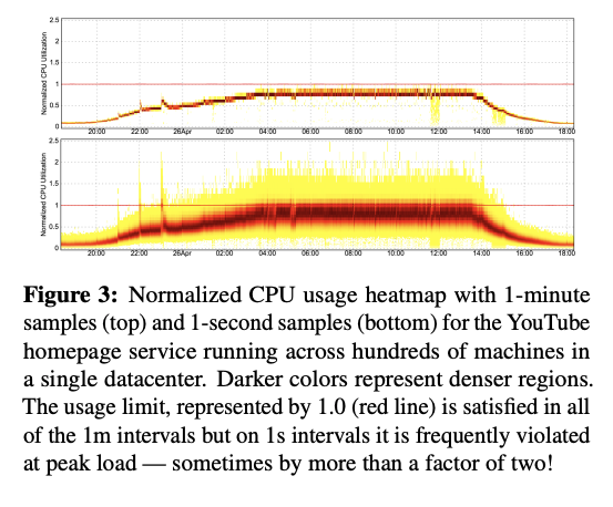
- CPU utilization might not be overloaded in the timeframe of 1 minute, however, if we zoom into the 1 second timeframes, we’ll be able to see that it’s an illusion! (Check the image below)

Enough of the background, let’s dive into the algorithm.
Asynchronous Client-Side Probing
- Each client powered by prequel has a pool of $n$ servers that it probes at a rate of $r_{probe}$. In the paper, these probes are triggered by either on a query or a specificed maximum idle time interval. In my implementation, I’ve chosen an option 3, that is, A specific time interval, independent of the query rate. Each probe aims to fetch the following metrics from the server:
- RIF - Use server’s current counter (simple atomic counter should do)
- Latency - Should be tagged with server’s current counter as well.
- The paper suggests that out of the $n$ servers, the client should pick a random set with uniform distribution to avoid thundering herd. I have kept it simple in mine and went ahead with sampling all of them (considering we are only sampling 5 of them).
- The probe pool should be maintained at a fixed size of $16$. It’s responsible for storing the probe results from the servers.
- After each probe, the client will additionally maintain the distribution of RIFs. The paper, unfortunately, doesn’t shed light on what kind of distributions, so I’ve chosen a simple normalization. I have monitored the $RIF_\text{max}$ received across servers and just divided $RIF_\text{curr}$ with the $RIF_\text{max}$ to get normalized values. This will be used later in server selection.
Server Selection
On each query, the prequel powered load balance will employ HCL (Hot Cold Lexicographic) to select the server. Each client maintains a RIF quantile ($Q_\text{RIF} \in [0.6, 0.9]$).
A server $s$ is hot if the distribtuion of RIF follows $ RIF_\text{s} \geq Q_\text{RIF}$, else it’s cold.
- If all servers are hot, then it picks the one with lowest latency among them.
- Else, pick any cool server for serving the said request.
Probe health at client level
- A probe may be too old, too overused or simply depleted to be used for the server estimation.
- To ensure we have staved off some probes without increasing $r_{probe}$, we extend the life of a probe by reusing up to $b_{reuse}$ time where $b_{reuse}$ is calculated via (where $\delta > 0$, $m$ is the max probe pool size and $n$ is number of servers) -
- Additionally, there should be a time limit for the probes to be reused. In my implementation, that’s configurable.
- Apart from the problems above, there’s an interesting case of degradation, how does that occur?
- If the client keeps picking up probes which have light load (as it should), then we would keep removing these probes after some reuse, and whatever’s left will be probes of server with heavy loads.
- This would be solved by the periodic removal of loads. Now, how will it remove one?
- If there is any probe which is hot, the the hot probe with highest RIF will be removed.
- Else, a cold probe with highest latency will be removed.
Server Metrics Estimation
Naturally, a fun question pops out, these metrics are served by the server, but how?
- The RIF is served by an Atomic Counter.
- The Latency is served slightly differently.
- After each query, server stores the latency and tags it with the observed RIF at the start of the query.
- When a probe arrives, it fetches the median latency for the nearest $k$ RIFs which is closest to server’s current RIF (Let’s call this $RIF_{curr}$).
- In my implementation, I’ve chosen $k = 10$ while maintaining a pool of $1000$ samples.
My Experiments
For my experiment, I have done the following:
- Run all 5 servers with no prior load, run the Prequel backed client and observe the traffic. The client will be serving requests at the rate of 100 RPS.
- Run a new Round Robin LB backed client for server 1,3 and 5, observe.
- Run a new Round Robin LB backed client for servers 2 and 4 observe!
All screenshots are from prometheus :D
Observations
Checkpoint 1
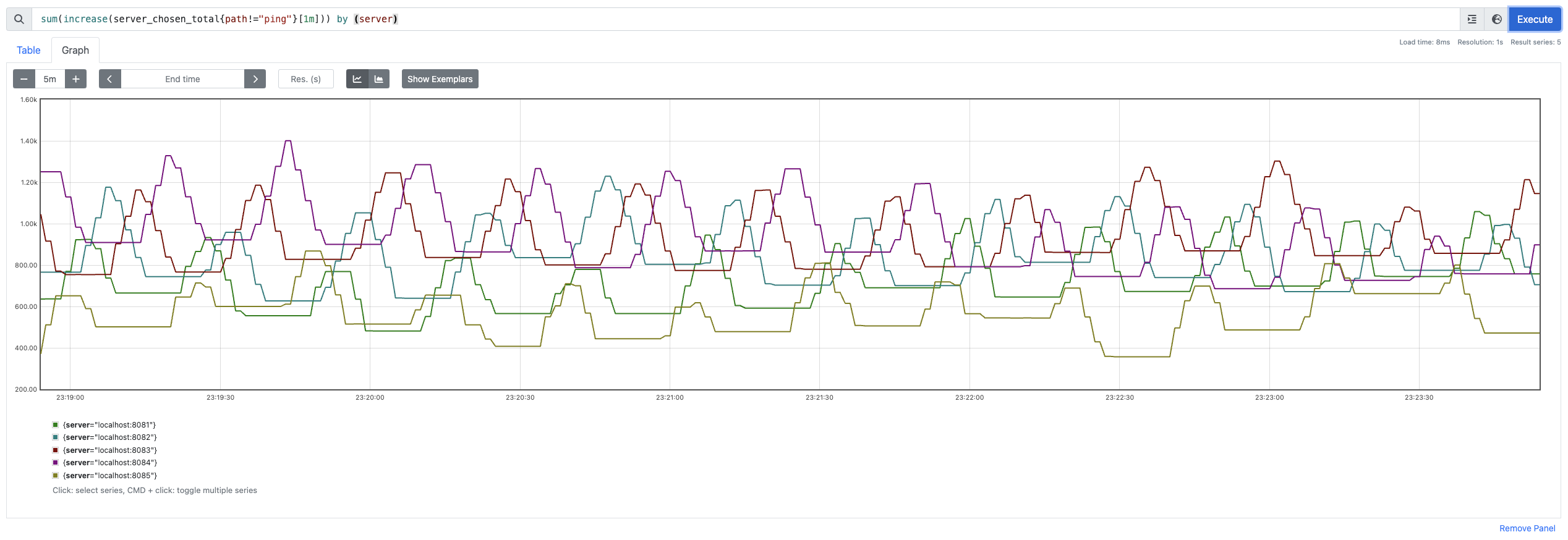
With only one client, we can notice all the servers getting comparable requests with maximum served to localhost:8083 ($1200$) and minimum served to localhost:8085 ($470$).

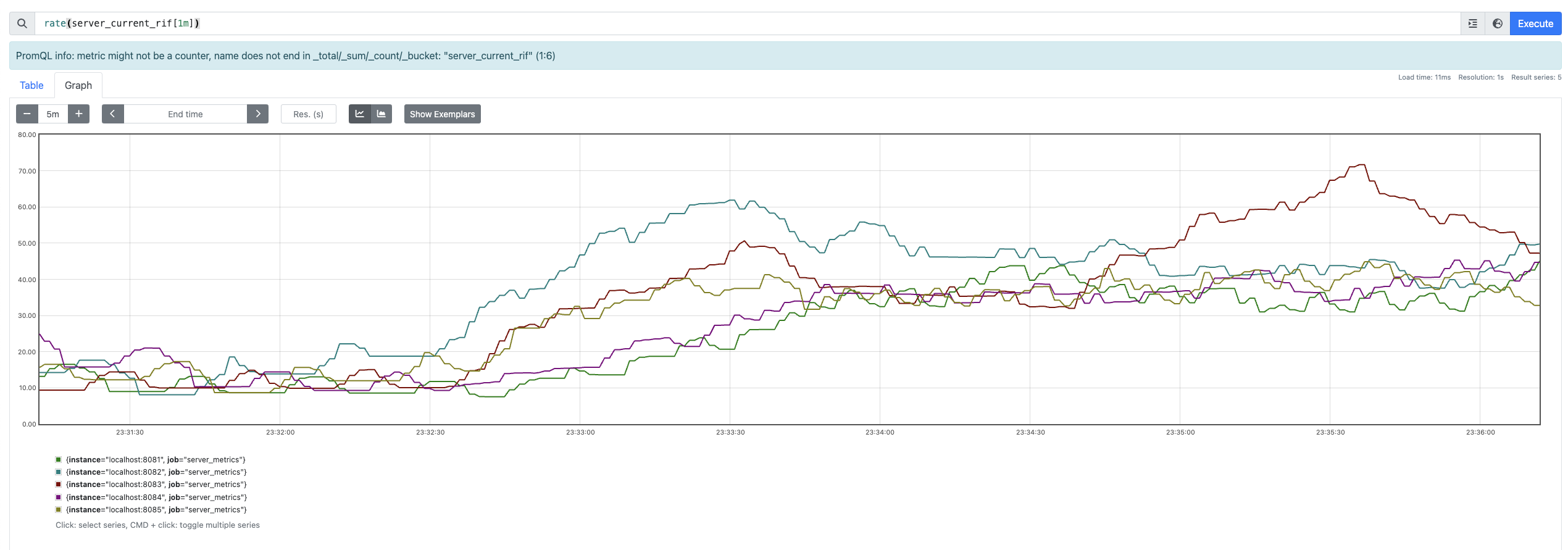
This is supported by the fact that, for some reason, the normalized value of the probe at localhost:8083 is 0.

Checkpoint 2
In this checkpoint, let’s bump up the traffic for servers served at :8083, :8084 and :8082 with round robin load balancers.
You’ll notice that the client immediately prioritizes sending requests to the less loaded servers :8081 and :8085 while dropping the traffic to the hot servers to almost 0!

However, the server traffics raises fairly linearly thoughtout all the servers. This is because all of them are serving one client or the other.

Interestingly, it seems that even in cold shard scenario, my implementation is prioritizing loads with low median latency because the distribution of $RIF_s$ is quite comparable.

It’ll be interesting to see if the loads balance if we start a new client serving to the rest of the 2 servers.
Checkpoint 3
Surprisingly (or is it?) the traffic being served to the 2 healthier servers has suddenly decreased!

Does it make sense though? Indeed it does, the new round robing is pushing ~500 RPS on these 2 servers however the earlier 3 servers are serving only ~333 RPS per. (Note, it’s 1000 RPS being distributed among $n$ servers per script). Hence, the median latency is increased for these 2 servers.
Interestingly, as per the probe distribution, the RIF stays the highest for localhost:8083 (might be a bug in implementation, it's entirely based on presumption after all).

Throughout the expirement you’ll notice that HCL prioritized serving the request to a cold server!

My experiments could be extended with various other parameters like, different processing times, different distribution techniques, dynamic $Q_\text{REF}$ calculation and have fun with it :D
Conclusion
I loved the simplicity and the description provided in paper for the said distributions. You could tell that utilizing the RIFs as the primary factor has served the tail latencies well, you could infact, keep the $Q_\text{RIF} = 0$ and still observe amazing results.
The paper also talks about a synchronous probing technique, which is well explained there, hence didn’t feel the need to expand on the same.
Hope you had fun with the load balancer metrics.
Merry Christmas to those who celebrate ^_^